Physics in games is always fun, isn't it? Have you ever ditched the main quest of a level just to blow something up? I know I have.

But even more fun than watching objects bounce around the screen is to understand how we can use simple concepts from high-school mathematics to simulate those physics laws with code.

This article is divided into the following sections:

• The basics of physics simulation
• A quick review of differentiation and integration
• Numerical integration in the context of motion
• Euler Integration
• Verlet Integration
• JavaScript implementation of Verlet integration
• C++ implementation of cloth simulation

And this is still a tiny subset of what we understand by game physics. Our main goal is to explore something called Verlet integration. We'll look at its motivations, intuition, and how we can use Verlet integration to write a simple 2D cloth simulation with C++.

Oh, and if you ever asked yourself why your university required you to take Calculus as a CS student, this blog post might help you answer that question as well.

Physics Simulation is a Discrete Game

Simulating physics with a computer requires us to compute things like forces, acceleration, velocity, and position in discrete time steps. We need a way of predicting the new position of an object on the screen for each time step.

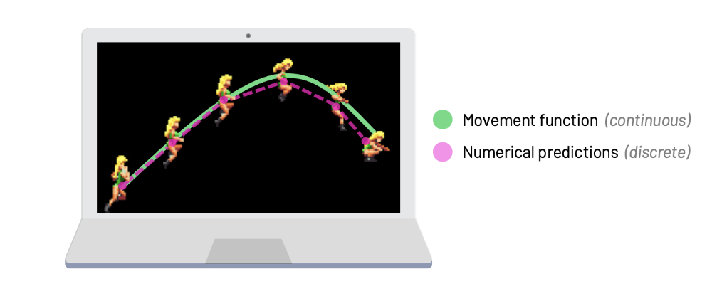
As it turns out, there are several methods we can use to find these predictions. Some prediction methods are faster, some are more stable, and some are expensive but give better approximations. Depending on the type of problem we are simulating, we can make educated guesses on which prediction method we should pick.

You will hear some programmers use the term integration when talking about these predictions. Some popular integration techniques used by physics programmers are Euler's method, Runge-Kutta methods, and of course, Verlet integration.

If you ever took Calculus before and you got scared by the word "integration", don't worry! We'll review the basics to make sure everyone is on the same page.

Why Verlet?

Verlet integration gets its name after the French physicist Loup Verlet. Verlet used this method of integration in his article Computer "Experiments" on Classical Fluids, I. Thermodynamical Properties of Lennard-Jones Molecules, published in July of 1967. However, it's believed that it was first used by Delambre in 1791, and has been rediscovered several times since then. You'll also read books that use the name Störmer's method for this technique (by Carl Størmer). In this post, I'm going to stick with the common term "Verlet integration".

These days, Verlet Integration plays an important role in many game physics engines. It's less expensive than, for example, Runge-Kutta methods (though also less accurate), but it's also much more stable than Euler's method. Its stability makes this method ideal especially for simulations with moving parts where each has certain degree of freedom, but all are connected together, so each also influence the others either directly or indirectly. You'll see that our article describes a cloth simulation that consists of points connected with sticks (constraints), which is exactly the type of scenario that benefits from Verlet's stability!

Different types of physics engines can benefit from choosing different integration methods. For example, Euler integration is a popular choice for rigid-body physics. Rigid-body engines simplify the problem by assuming the shapes of our objects can never change or deform. For this type of scenario, Euler integration gives good-enough approximations and it's reasonably stable.

Alright! Before we dive in, I'd like to mention one super important thing. I could've just started with a brief explanation of how Verlet integration works a then walk you through the code and that would be probably fine for most people. Maybe you already know the basics of integration & differentiation and understand what I mean when I talk about stability, accuracy, and expensiveness in the context of physics simulation. If you remember all this stuff from university or even from the 2D Game Physics Programming course here at pikuma.com, then I think you can skip the following section and continue from the part titled "Numerical Integration of Equations of Motion".

However, I really want this post to be for people who never encountered these sorts of things before, or simply forgot because they never used it outside their math class. That's why I added a chapter called "Integration and Differentiation 101", where anyone can learn the very basics (but enough) of the underlying theory to better understand the rest of this article.

Integration and Differentiation 101

Many of us were forced to spend an entire semester learning about integration and differentiation in college. Some degrees even break these topics into several modules, like Calculus I, Calculus II, Calculus III, etc. Nowadays, you can find online books that will guide you in the journey of learning calculus, or you can even start by watching a beginner-friendly online video if you want to start learning this at your own pace.

Here, I'm going to cover just those bits of theory I think are essential for our use case. Though I wanted this post to be a practical one, just throwing code at you without explaining any of the underlying theory doesn't feel right.

I also think the explanation of the basics of integration is not complete without at least a brief talk about its opposite, the differentiation. Bear with me, it'll be really quick.

Differentiation

Let's say we have a simple quadratic function, \(f(x)=2x^2\). Think of this as a function that defines the movement of a player in a game, for example. And let's also say want to find the slope of this function between the values \(x=1\) and \(x=2\).

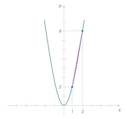
It's simple, right? We calculate the result of the function at \(x=1\) and \(x=2\), which gives us \(f(1)=2\) and \(f(2)=8\), and we then proceed to calculate the difference of these outputs to get the slope for the interval we want.

For one unit of x, our y value grows 6 units. Therefore, we can say that this slope value tells us the average rate of change for a range of values of our function. I chose the terms "average" and "rate of change" very carefuly here, and you'll understand why soon.

Sometimes I like to put things into context and translate math into something I can relate to. So, instead of using terms like function and slope, try thinking of how fast an enemy is moving in pixels per frame/update of our game. In the example above, we could imagine that the average rate of change of the position of our enemy was 6 pixels between steps 1 and 2 of our simulation.

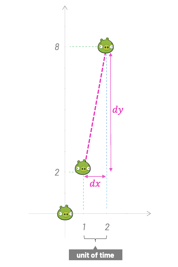
Now, let's say we do not want the average rate of change. Instead, we are interested in the instantaneous rate of change at a single point of our function. Well, following the same approach, both \(dx\) and \(dy\) will be 0, and 0/0 has no meaning.

Before we solve that problem, let's go even a bit further. We don't want to find the slope for a single point, but for any point of our function. We want another function that tells us how the output of the function \(f(x)\) changes for any given \(x\).

This function is called the first derivative, and to find this first derivative of \(f(x)=2x^2\) we're going to use something called differentiation.

How do we do it? First we agree that both \(dx\) and \(dy\) are infinitesimals (infinitely small) but not zero. In other words, they approach zero. Sometimes you'll see \(dx\) and \(dy\) written as \(\Delta x\) and \(\Delta y\), where \(\Delta\) is the uppercase Greek letter delta. In math, the \(\Delta\) symbol usually means "change".

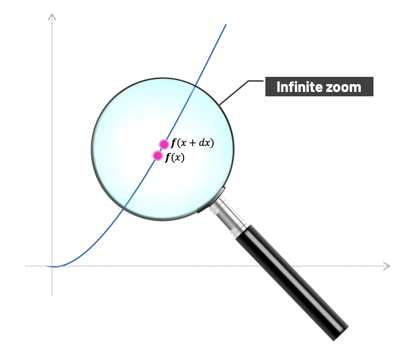
The general approach to finding derivatives doesn't differ that much from what we've already done when we had two discrete points. If we'd add an "infinitesimal amount" \(dx\) to \(x\) and zoom infinitely, we'd see \(x\) and \(x+dx\) as two points, just as before. The distance between them is infinitesimal, but the great thing about our minds is they are not limited as the real world is, and that's the beauty of abstract ideas; we can imagine we zoomed infinitely to see the distance. It's almost like having a super-power!

And now we can do almost the same as we've done before. Only this time, our calculation would be general.

We have our original function:

If we add that infinitesimal amount \(dx\) to \(x\), we get:

As I mentioned before, the logic is basically still the same as when we were calculating the average rate of change between two discrete points. We simply get on the left side:

And on the right side:

We can now proceed to simplify the right hand side using algebra:

\(=\frac{2(x^2+2x.dx+dx^2)-2x^2}{dx}\)

\(=\frac{2x^2+4x.dx+2dx^2-2x^2}{dx}\)

\(=\frac{4x.dx+2dx^2}{dx}\)

\(=4x+2dx\)

\(=4x\)

In the last step, we just got rid of \(2dx\) because it approaches zero; and since it's almost nothing, we treat it like nothing. We could've done that sooner, but I wanted to show the process one step at a time.

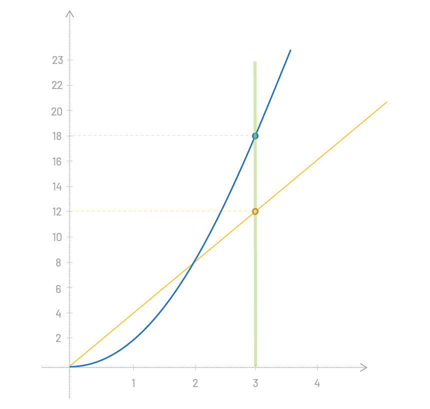
And now comes the beautiful part. Since we just found out that the first derivative \(f'(x)\) is \(4x\), we can calculate the slope at any point of the original function \(f(x)=2x^2\).

For example, for \(x=3\), the output is \(f(3)=18\), and the slope is \(f'(3)=4*3=12\).

We can visualize that as we plot both functions and draw a vertical line parallel with the vertical axis at \(x=3\).

There's a faster way to find that the first derivative of \(f(x)=2x^2\) is \(f'(x)=4x\). You can probably guess the rule if I tell you that the first derivative of \(x^2=2x\) and the first derivative of \(3x^2=6x\).

A big part of any Calculus class revolves around these diferentiation rules. There are lists of rules for different functions that super smart people discovered a long time ago. The rule above is probably the easiest one to remember, where the first derivative of any function of the form \(Ax^B\) is always \(BAx^{B-1}\).

We can go even further. The second derivative is the result of the differentiation of the first derivative. In this case it is a constant; the number 4. You may have noticed that the derivative of a quadratic function is a linear function, and derivative of a linear function is a constant. If you did, great job!

Alright! That's as far as I want to go with differentiation. My goal here was not to teach differentiation; this are just the basics anyway. What I aimed for is to build an intuition that will be useful later. Let's go ahead and do the same for the integration.

Integration

Again, we're going to cover just the most basic example. Bear with me; even that will help you understand the rest of the article much better, especially if all this is new for you.

Integration and differentiation are inverse operations. Integration can be useful when we need to calculate an area or a volume. Let's illustrate the process of integration with a simple example.

Let's say we have a function, \(f(x)=2x\) and want to calculate the area under the function for the slice between \(x=0\) and \(x=4\).

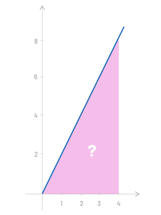
Right... so, for this particular example you probably already see that we can just calculate the area of a triangle \((4*8)/2=16\). We have our result. Easy!

But how about if I ask you to find the area under the function \(f(x)=sin(3x^2)\) for the slice between \(x=0\) and \(x=1.023\)?

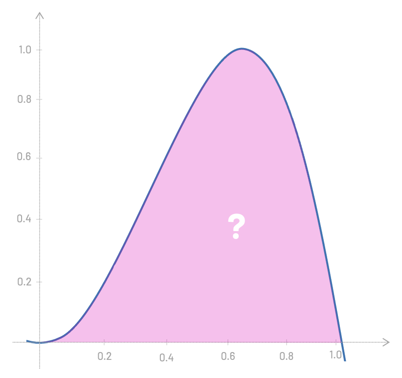
Well, that's a little bit more complicated. But one thing we could do here is to get an approximate result by breaking the area into rectangles and summing all of their areas. For this example, that would be (0.2 * 0.2) + (0.2 * 0.4) + (0.2 * 0.8) + ..., you get the idea.

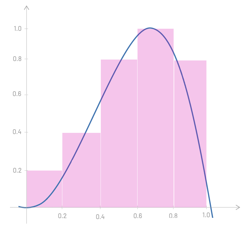
However, this approximation is not very good; our rectangles are too wide. If we make them narrower, we get a better approximation.

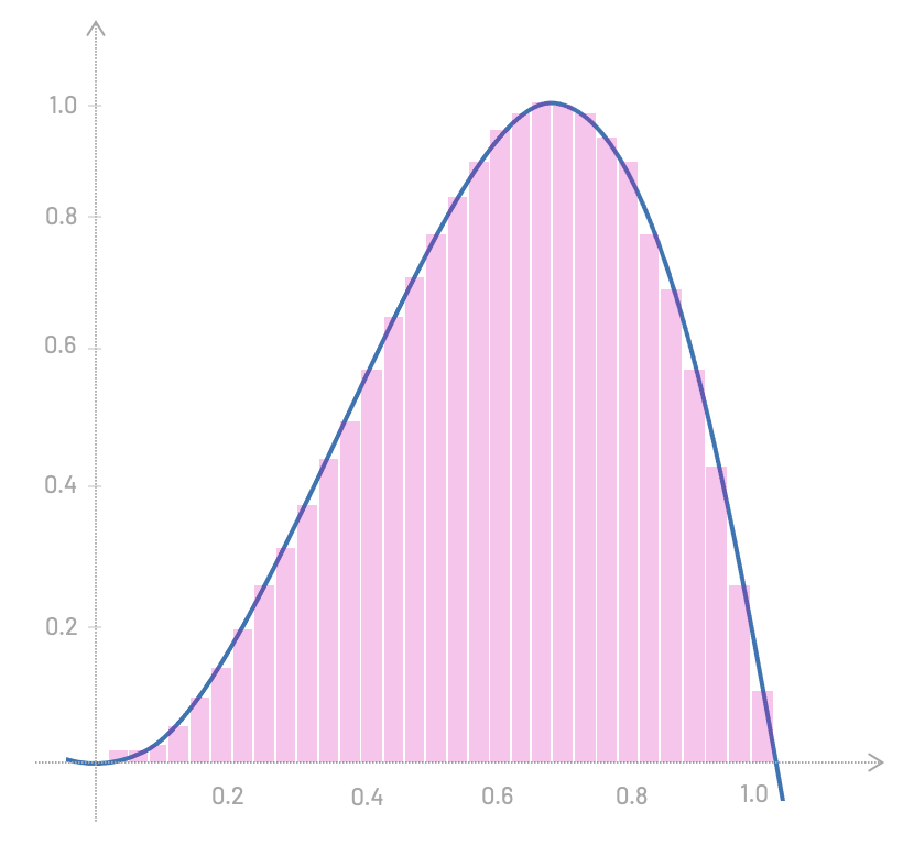
And the less wide they are, the more accurate our result gets.

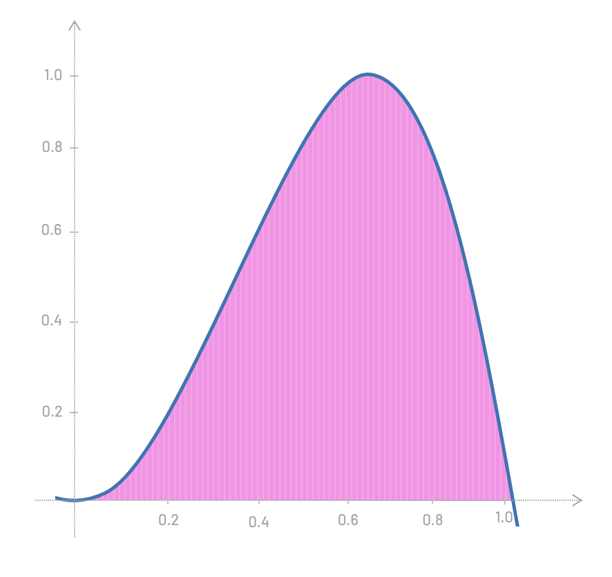
You probably already know where we're heading, right? What if we make the width of these rectangles infinitesimally small?

Let's get back to our linear function \(f(x)=2x\) and let me also introduce the \(\int\) symbol, which is stylized S, for "Sum".

Formally, we can write the idea of integration of this function like this:

Let's quickly break this notation apart and analyze its parts. The \(\int\) is the Integral symbol, \(2x\) is the actual function we want to integrate, \(dx\) is the infinitesimal slice along which we integrate, and \(C\) is the integration constant, which I'll soon explain.

This time, let's also make our life easier and integrate this function using one of the antiderivative rules that have been discovered and proved right a long time ago.

In this example, we'll use two rules:

• First, the Power Rule, because we have \(x\) and this is the same as \(x^1\).
• Second, the Multiplication by Constant Rule, because we are multiplying \(x\) by 2.

In most math books, these two rules stands like this, respectively:

	\(1.\;\int{x^n \; dn} = \frac{x^{n+1}}{n+1}+C\)
	\(2.\;\int{k \; f(x) \; dx} = k\;\int{fx\;dx}\)

The good news is that our example, \(f(x)=2x\), meets both conditions. We are making sure \(n\) is different than \(-1\) (from \(x^1\)), and the scalar 2 is, indeed, a real number (\(k \in \mathbb{R}\)). We can proceed with our integration!

We first use the multiplication by constant rule, pulling the scalar 2 outside the integral:

And then, the power rule:

\(2\int{x \; dx}\)

\(=2 \left( \frac{x^{1+1}}{1+1} \right) + C\)

\(=\frac{2x^2}{2} + C\)

\(=x^2 + C\)

We just found out that the integral of \(f(x)=2x\) is given by \(x^2+C\).

Now, I think it's a good time to explain what the integration constant \(C\) is. The term \(+C\) simply sums up the idea that no matter what expression you add to \(x^2\), its first derivative will always be \(2x\).

If we take the function \(f'(x)=4x\) and we integrate it, we'll get back to \(f(x)=2x^2\). That's why we say integration and differentiation are inverse operations.

Again, these are just the very basics of differentiation and integration, and you can spend many months exploring this topic. You'd learn different rules to analytically solve derivatives and integrals; you'd also learn about limits (which we barely touched here), you'd learn the L'Hôpital's rule, chain rule, etc. As I wrote before, this is not our goal here.

Let's now procceed to the next section, where we'll be talking about Euler integration and Verlet integration. We'll learn how they differ from each other, and I believe that even with this very basic knowledge of integration and differentiation, you'd understand what comes next much more easily.

And even later, when I'll guide you through an implementation of a cloth simulation, knowing the underlying theory, to wrap your head around the code wouldn't be just easier, but also more fun!

Numerical Integration of Equations of Motion

Beautiful! Let's resume talking about physics simulation.

You probably remember from high school one of Newton's laws of motion that tells us that the force of a sysem is equals the mass times the acceleration. I'm positive you've seen this formula before.

Therefore, if we know the total force and we know the mass, we can just move things around to find the acceleration:

This formula makes sense, intuitively, because if you kick a light ball, it accelerates; but if you kick a heavy car, it won't move a bit (but you may break your leg).

And here is where our review of derivatives and integrals starts to pay off.

Acceleration is the first derivative of the velocity with respect to time.

Similarly, the velocity is the first derivative of the position with respect to time.

This should all make sense, since velocity is the rate of change of the position through time, and acceleration is the rate of change of the velocity through time.

Euler Integration

Let's hit the ground running and write a short script to simulate the movement of a single particle in 1 dimension.

We start by encapsulating some default values in a Particle class. This particle will have position, mass, and velocity. By using Newton's laws of motion, we'll be applying a force to update the velocity and the position of the particle ten times with a while loop. This will be done in time steps, from 0 to 10.

class Particle {
  constructor() {
    this.position = 0.0;
    this.velocity = 0.0;
    this.mass = 1.0;
  }
}

function main() {
  let particle = new Particle();

  let force = 10.0;
  let acceleration = force / particle.mass;

  let time = 0.0;
  let deltaTime = 1.0;
  
  while (time <= 10.0) {
    particle.velocity += acceleration * deltaTime;
    particle.position += particle.velocity * deltaTime;

    time += deltaTime;
  }
}

If we print out the position and velocity at every step, we get the following results:

time = 0    position = 0      velocity = 0
time = 1    position = 10     velocity = 10
time = 2    position = 30     velocity = 20
time = 3    position = 60     velocity = 30
time = 4    position = 100    velocity = 40
time = 5    position = 150    velocity = 50
time = 6    position = 210    velocity = 60
time = 7    position = 280    velocity = 70
time = 8    position = 360    velocity = 80
time = 9    position = 450    velocity = 90
time = 10   position = 550    velocity = 100

What we've done here inside this while loop is something called Euler Integration. This method is named after the Swiss mathematician, physicist, astronomer, geographer, logician, and engineer (remarkable person, really) Leonhard Euler (pronounced [/'ɔɪlər/]).

This approach is simple and very intuitive. We always adjust the change in velocity and position by a delta time factor. In the example above, deltaTime was set to a fixed value of 1.0, but the values of deltaTime can be bigger, smaller, and even different from one time step to the next.

However, computer simulations don't run in a perfect world of ideas where we can have infinitesimal time steps. For computers, time generally runs in discrete cycles. In fact, can we decide whether time in our universe is continuous or discrete? Ticking one Planck time at a time sounds paradoxical, right? Maybe it's both, somehow. That's not a trivial question and one can spend a lifetime thinking about that.

Let's get back to our simple simulation. As I mentioned, time in our simulation runs in discrete steps, which means the results of such a numerical integration wound never be precise. If we calculate the position using the closed-form of the constant accelerated motion formula for t = 10, using the same initial values of velocity = 0, and acceleration being force divided by mass (10/1 = 10), we'll get the correct result 500; not 550.

\(dx=v_0 t+\frac{1}{2}at^2\)

\(dx=0+\frac{1}{2}(10)(10)^2\)

\(dx=500\)

The bigger the time step is, the bigger error we get. Remember those wide slices in the previous discussion about integration, when we were talking about calculating the area under the function.

Let's try to solve this issue using a much smaller time step.

let deltaTime = 0.01;

Instead of 10 iterations, let's now run 1000 times. The results for t = 10 would be much more accurate. Unfortunately, the calculation will now take 100 times longer.

time = 10    position = 500.498    velocity = 99.999

The other bad news is that the error is also cumulative. The longer the simulation runs, the bigger our error gets. We can see the difference if we run the simulation 100 times longer.

while (time <= 1000) {
  /* ... */
}

After 100,000 iterations, the error is much bigger than before; even with the same time step of 0.01. The correct position should have been 5,000,000.00.

time = 1000    position = 4,995,430.500    velocity = 9991.982

Alright. Let's leave Euler integration and finally move to Verlet integration.

Verlet Integration

Now that we learned about Euler integration, let's move forward and discuss Verlet integration.

For this next example, I would like to have some visual feedback. Instead of just printing values in the console, let's take advantage of a graphics library called p5.js. You can either manually download the p5.js library, or simply follow along using the online p5js web editor (editor.p5js.org).

When you paste the following code to the p5.js editor and hit the play button, you should see four small white circles falling and slowly accelerating.

class Particle {
  constructor(x, y, mass) {
    this.x = x;
    this.y = y;
    this.prevx = x;
    this.prevy = y;
    this.mass = mass;
  }  
}

let particles = [];

function setup() {
  createCanvas(500, 400);
  let pA = new Particle(220, 20, 10000);
  let pB = new Particle(280, 20, 10000);
  let pC = new Particle(280, 60, 10000);
  let pD = new Particle(220, 60, 10000);
  particles.push(pA, pB, pC, pD);
}

function update() {  
  for (let i = 0; i < particles.length; i++) {
    let particle = particles[i];
  
    let force = {x: 0.0, y: 0.5};
    
    let acceleration = {x: force.x / particle.mass, y: force.y / particle.mass};
    
    let prevPosition = {x: particle.x, y: particle.y};

    particle.x = 2 * particle.x - particle.prevx + acceleration.x * (deltaTime * deltaTime);
    particle.y = 2 * particle.y - particle.prevy + acceleration.y * (deltaTime * deltaTime);
    
    particle.prevx = prevPosition.x;
    particle.prevy = prevPosition.y;
  }
}

function draw() {
  background(0);
  
  update();
  
  for (let i = 0; i < particles.length; i++) {
    circle(particles[i].x, particles[i].y, 10);
  }
}

As we run our simulation, we can see four particles falling and updating their position frame by frame. Here, we are using Verlet integration to predict the new position of the particles at each time step.

So what's going on here? First, we create a Particle class, and then proceed to declare a global array of particle objects.

let particles = [];

The setup() function is called automatically by P5.js at the beginning of the execution. Here is where we create a new canvas and add the four particle objects to our array.

function setup() {
  createCanvas(500, 400);
  let pA = new Particle(220, 20, 10000);
  let pB = new Particle(280, 20, 10000);
  let pC = new Particle(280, 60, 10000);
  let pD = new Particle(220, 60, 10000);
  particles.push(pA, pB, pC, pD);
}

Unlike in the previous 1D example, we are not storing the velocity of the particle. We store only the current position (x,y), the previous position (prevx, and prevy), and the mass of the particle.

Storing this previous position is the heart of Verlet integration!

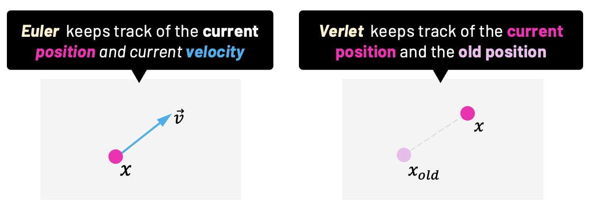
With Verlet, the velocity is "given" by the difference between the current and the previous position. We'll get more into that in a moment. For now, just note how we are assigning the same value to both current and previous position in the constructor, since we don't want any initial velocity.

class Particle {
  constructor(x, y, mass) {
    this.x = x;
    this.y = y;
    this.prevx = x;
    this.prevy = y;
    this.mass = mass;
  }
}

In the update() function, we loop all particles to store the current position of the particle to a temporary variable. We define a value for the force and we proceed to calculate the acceleration using Newton's formula, \(a=F/m\).

And here is where Verlet integration does its magic! The new current position is based on the previous position multiplied by 2, the acceleration, and the deltaTime squared.

This is the Verlet integration:

After that, we set the previous position from our previously saved variable (where the current position was stored before the integration).

function update() {  
  for (let i = 0; i < particles.length; i++) {
    let particle = particles[i];
  
    let force = {x: 0.0, y: 0.5};
    
    let acceleration = {x: force.x / particle.mass, y: force.y / particle.mass};
    
    let prevPosition = {x: particle.x, y: particle.y};

    particle.x = 2 * particle.x - particle.prevx + acceleration.x * (deltaTime * deltaTime);
    particle.y = 2 * particle.y - particle.prevy + acceleration.y * (deltaTime * deltaTime);
    
    particle.prevx = prevPosition.x;
    particle.prevy = prevPosition.y;
  }
}

And just to conclude, the last part is simply the call of the p5.js draw() function (which is called several times per second). Here is where we ask to update our particles and also render the circles on the screen for each particle using the circle() function from p5.js.

As you can see, there's been a lot of work already done for us by P5.js; it's a handy tool for such quick demonstrations. Let's make some last changes before we finally dive into cloth simulation using Verlet.

Because we don't want to go down the rabbit hole of having to properly handling collisions, we'll keep the particles inside the canvas with a little hack function called keepInsideView(). We'll simply test if their current position is outside the boundaries of the canvas; if it is, we stop the particle from moving. The width and height variables are provided by p5.js, and they are the width and the height of our 500x400 canvas.

function keepInsideView(particle) {
  if (particle.y >= height) particle.y = height;
  if (particle.x >= width) particle.x = width;
  if (particle.y < 0) particle.y = 0;
  if (particle.x < 0) particle.x = 0;
}

function update() {  
  for (let i = 0; i < particles.length; i++) {
    let particle = particles[i];
  
    let force = {x: 0.0, y: 0.5};
    
    let acceleration = {x: force.x / particle.mass, y: force.y / particle.mass};
    
    let prevPosition = {x: particle.x, y: particle.y};

    particle.x = 2 * particle.x - particle.prevx + acceleration.x * (deltaTime * deltaTime);
    particle.y = 2 * particle.y - particle.prevy + acceleration.y * (deltaTime * deltaTime);
    
    particle.prevx = prevPosition.x;
    particle.prevy = prevPosition.y;

    keepInsideView(particle);
  }
}

If we run the code now, we'll see what you expect. Four particles falling down that stop moving as they "hit the ground".

Constraints

But what if we want these points to keep the rectangular shape they have at the beginning? That's where the idea of a constraint comes in.

A constraint is another object that has references to a pair of connected particles and a length that should be maintained between them. In our example, I'll call our constraints "sticks". They'll behave exactly as sticks that connect the particles and maintain a hard distance between them.

We calculate their length according to the initial positions of the connected particles. In the update function, after iterating through particles and integrating their positions using Verlet integration, we'll also iterate through the constraints (sticks) and if the distance between particles after integration ends up being bigger or smaller than the initial length defined in the stick, we calculate the proper offset to alter the position of particles and thus maintain the initial length. To help us vizualize what's going on, we'll also draw a line for each stick inside the draw function.

class Particle {
  constructor(x, y, mass) {
    this.x = x;
    this.y = y;
    this.prevx = x;
    this.prevy = y;
    this.mass = mass;
  }  
}

class Stick {
  constructor(p1, p2, length) {
    this.p1 = p1;
    this.p2 = p2;
    this.length = length;
  }
}

let particles = [];
let sticks = [];

function getDistance(p1, p2) {
  let dx = p1.x - p2.x;
  let dy = p1.y - p2.y;
  return Math.sqrt(dx * dx + dy * dy);
}

function getLength(v) {
  return Math.sqrt(v.x * v.x + v.y * v.y)
}

function getDifference(p1, p2) {
  return {
    x: p1.x - p2.x,
    y: p1.y - p2.y
  };
}

function keepInsideView(particle) {
  if (particle.y >= height)
    particle.y = height;
  if (particle.x >= width)
    particle.x = width;
  if (particle.y < 0)
    particle.y = 0;
  if (particle.x < 0)
    particle.x = 0;
}

function setup() {
  createCanvas(500, 400);
  
  // Add four particles
  let pA = new Particle(220, 20, 10000);
  let pB = new Particle(280, 20, 10000);
  let pC = new Particle(280, 60, 10000);
  let pD = new Particle(220, 60, 10000);
  particles.push(pA, pB, pC, pD);
  
  // Add four stick constraints between particles
  let stickAB = new Stick(pA, pB, getDistance(pA, pB));
  let stickBC = new Stick(pB, pC, getDistance(pB, pC));
  let stickCD = new Stick(pC, pD, getDistance(pC, pD));
  let stickDA = new Stick(pD, pA, getDistance(pD, pA));
  sticks.push(stickAB, stickBC, stickCD, stickDA);
}

function update() {
  // Update particle position using Verlet integration
  for (let i = 0; i < particles.length; i++) {
    let particle = particles[i]

    let force = {x: 0.0, y: 0.5};

    let acceleration = {x: force.x / particle.mass, y: force.y / particle.mass};

    let prevPosition = {x: particle.x, y: particle.y};

    particle.x = 2 * particle.x - particle.prevx + acceleration.x * (deltaTime * deltaTime);
    particle.y = 2 * particle.y - particle.prevy + acceleration.y * (deltaTime * deltaTime);

    particle.prevx = prevPosition.x;
    particle.prevy = prevPosition.y;

    keepInsideView(particle);
  }

  // Apply stick constraint to particles
  for (let i = 0; i < sticks.length; i++) {
    let stick = sticks[i];

    let diff = getDifference(stick.p1, stick.p2);
    let diffFactor = (stick.length - getLength(diff)) / getLength(diff) * 0.5;
    let offset = {x: diff.x * diffFactor, y: diff.y * diffFactor};
    
    stick.p1.x += offset.x;
    stick.p1.y += offset.y;
    stick.p2.x -= offset.x;
    stick.p2.y -= offset.y;
  }
}

function draw() {
  background(0);
  
  update();
  
  for (let i = 0; i < particles.length; i++) {
    circle(particles[i].x, particles[i].y, 10);
  }

  for (let i = 0; i < sticks.length; i++) {
    stroke("white");
    line(sticks[i].p1.x, sticks[i].p1.y, sticks[i].p2.x, sticks[i].p2.y);
  }
}

Notice how we added a few helper functions in our code. The function getDifference subtracts the x and y coordinates of two points and return the results. We have also the functions getLength and getDistance, in which we use the Pythagorean theorem to calculate the length of a vector and the distance between to points, respectively.

We should see once again 4 falling particles, but this time they should be connected with sticks (constraints). Once the bottom line touches the ground, the square maintains its shape for a while, and then it folds to one side.

What do we need to do to keep the square shape all the time? That's right; we'll have to add other sticks between particles pA and pC, and pB and pD. I'll leave that for you as a small exercise.

Believe it or not, now you know all the theory behind the type of cloth simulation we'll use in this article. This is because our implementation will be nothing more than an array of particles with stick constraints that keep them together. However, in the next section, besides walking you through this implementation of a simple cloth simulation, I'll also show you how we can handle mouse input to drag and tear the cloth.

The good news is that, because now you know all the underlying theory, I guarantee you won't have a hard time understanding the implementation.

Coding a 2D Cloth Simulation

We'll now cover the implementation of the cloth simulation in C++. I'll also show you how mouse inputs are handled to drag and tear the cloth, and thus you'll also learn a bit about SDL (Simple DirectMedia Layer) if you've never worked with this library before.

One of the main reasons we are moving away from JavaScript is because C++ forces us to think about some low-level details of our application. For example, some small things that we took for granted using JavaScript (like its gameloop or automatic memory management), we'll have to create manually with C++. And that's a good thing, since we want to learn how things really work!

You can find the implementation I'm going to walk you through in this GitHub repository. We'll go together through every class, and I'll explain in detail the parts that are essential. Let's start at the very top layer, in the Main.cpp file.

#include <iostream>
#include <math.h>
#include "Application.h"

int main(int argc, char* args[]) {
  Application app;
  app.Setup(1200, 320, 10);

  while (app.IsRunning()) {
    app.Input();
    app.Update();
    app.Render();
  }
    
  app.Destroy();
  return 0;
}

We have an app instance of the Application class, which encapsulates the logic of the entire application. This could've been named World or Environment, and that would make sense too.

Next, we call this Setup function to prepare the application. Then, we have a very simple "game loop" where we gather user input (mouse and keyboard events), update the application's state, and also draw the current state of our application to the screen. This is the holy trinity of the game loop: input, update, and render.

A single execution of such a loop is often called a frame or a step. I'll stick with the term frame, and I'll use step for the three steps (input, update, render) in one frame.

These three main steps are executed over and over, frame by frame, unless IsRunning is false, which happens when the user presses the ESCAPE key. Before the very end, the Destroy function frees the memory that has been allocated for internal objects that were created using the C++ keyword new.

Let's now look into the Application.h header file.

#include <vector>
#include "Mouse.h"
#include "Renderer.h"
#include "Cloth.h"

struct Application {
  private:
    Renderer* renderer = nullptr;
    Mouse* mouse = nullptr;
    Cloth* cloth = nullptr;

    bool isRunning = false;

    Uint32 lastUpdateTime;

  public:
    Application() = default;
    ~Application() = default;
  
    bool IsRunning() const;

    void Setup(int clothWidth, int clothHeight, int clothSpacing);
    void Input();
    void Update();
    void Render() const;
    
    void Destroy();
};

The first private member is a pointer to an SDL Renderer. The Renderer class is just a thin wrapper around SDL. We pass the pointer to a renderer instance down to Cloth and subsequently to Stick to render lines between connected Points. You already have an idea about how Sticks and Points work from the previous examples with p5.js. Previously, we used the term Particle instead of Point, but they are essentially the same thing here. We also use SDL to gather inputs in the Input function, and we'll get to that soon.

If the SDL library is new for you, I encourage you to open the SDL Wiki to read the basics of what SDL can do for us. You can also examine both Renderer.h and Renderer.cpp files on your own. For now, you can treat them as a black box that knows how to display graphics and render pixels on the screen.

Next, we have a pointer to Mouse. The instance of Mouse holds the position of our mouse cursor in both the current and previous frames. It will also keep for us information about which mouse buttons are pressed down and which are not.

We'll use this mouse information to apply forces to the points that are near the cursor. We'll do this to drag the cloth around when we press the left mouse button. We'll also be able to press the right mouse button to break constraints (sticks) between points, giving the impression of "tearing" our cloth.

Let's now just briefly look into the Mouse.h header file, to confirm these statements.

#include "Vec2.h"

class Mouse {
  private:
    Vec2 pos;
    Vec2 prevPos;

    float cursorSize = 20;
    float maxCursorSize = 100;
    float minCursorSize = 20;

    bool leftButtonDown = false;
    bool rightButtonDown = false;

  public:
    Mouse() = default;
    ~Mouse() = default;

    void UpdatePosition(int x, int y);
    const Vec2& GetPosition() const { return pos; }
    const Vec2& GetPreviousPosition() const {return prevPos; }

    bool GetLeftButtonDown() const { return leftButtonDown; }
    void SetLeftMouseButton(bool state) { this->leftButtonDown = state; }

    bool GetRightMouseButton() const { return rightButtonDown; }
    void SetRightMouseButton(bool state) { this->rightButtonDown = state; }

    void IncreaseCursorSize(float increment);
    float GetCursorSize() const { return cursorSize; }
};

I'll get back to this later when we'll be talking about how to properly handle input. For now, let's now head back to the Application class. Apart from the default constructor and destructor, other public functions we've already discussed, and isRunning flag, we have this lastUpdateTime member. We update and use this member variable to handle our deltaTime in the Update function. Remember how p5.js provided the deltaTime for us for free? This time, we have to calculate it ourselves, and we do it in the Update function.

void Application::Update() {	
  Uint32 currentTime = SDL_GetTicks();
  float deltaTime = (currentTime - lastUpdateTime) / 1000.0f;

  cloth->Update(renderer, mouse, deltaTime);

  lastUpdateTime = currentTime;
}

We just get the current time from an SDL function called SDL_GetTicks(). We subtract the last time from the current time, and at the end of the update, we save the current time as the last time for the next frame.

The most important thing that our Application class has is a pointer to an instance of Cloth. Let's open the Cloth.h file to see what this class is about.

#include <vector>
#include "Point.h"
#include "Stick.h"

class Cloth{
  private:
    Vec2 gravity = { 0.0f, 981.0f };
    float drag = 0.01f;
    float elasticity = 10.0f;

    std::vector points;
    std::vector sticks;

  public:
    Cloth() = default;
    Cloth(int width, int height, int spacing, int startX, int startY);
    ~Cloth();

    void Update(Renderer* renderer, Mouse* mouse, float deltaTime);
    void Draw(Renderer* renderer) const;
};

As you've probably expected, our cloth consists of multiple points connected with sticks (constraints). We store all the cloth's points and sticks in C++ vectors (similar to a JavaScript dynamic array). We also keep the gravity, drag, and elasticity here, which we'll later pass to each point to be used by our integration.

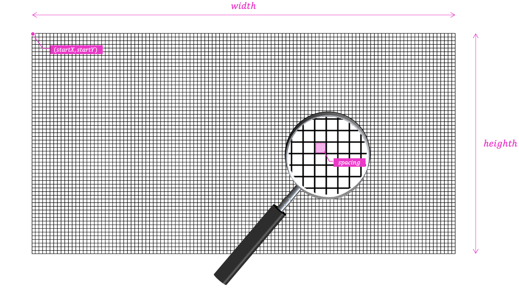
If you look at the public functions, you'll see we pass the width and the height of our cloth to the parameterized constructor. We also pass the spacing, which is the original distance from one point to another (or the distance that a stick should maintain between two points). We already saw how this works in the last p5.js example with the box made of four interconnected points. We also pass the starting position of our cloth, its top-left corner, startX and startY.

Let's briefly examine the Application's Setup() function, where the Cloth constructor is called.

void Application::Setup(int clothWidth, int clothHeight, int clothSpacing) {
  renderer = new Renderer();
  mouse = new Mouse();
  
  isRunning = renderer->Setup();

  clothWidth /= clothSpacing;
  clothHeight /= clothSpacing;
  
  int startX = renderer->GetWindowWidth() * 0.5f - clothWidth * clothSpacing * 0.5f;
  int startY = renderer->GetWindowHeight() * 0.1f;

  cloth = new Cloth(clothWidth, clothHeight, clothSpacing, startX, startY);

  lastUpdateTime = SDL_GetTicks();
}

Here, we create a new SDL Renderer and a new Mouse instance; we talked about both of them previously. Then, we call Setup on the renderer instance to create an SDL window and an SDL renderer. I just want to mention that, if there's no error, the renderer Setup function will return true. We use this boolean value to signal the application it can safely run.

Then we calculate the startX and startY positions of our Cloth based on the clothWidth, clothHeight, clothSpacing, and the size of our SDL window. We want our cloth to start horizontally centered in the window and vertically by 10% from the top.

After we create a cloth and we pass the calculated values to the Cloth constructor, we assign the current time from SDL_GetTicks() to lastUpdateTime. If we don't do that, our first deltaTime value that was calculated in the Update function would be off, causing a nasty lag.

Now, let's look into the Cloth constructor, where we effectively add all the points and connect them with stick constraints.

Cloth::Cloth(int width, int height, int spacing, int startX, int startY) {
  for (int y = 0; y <= height; y++) {
    for (int x = 0; x <= width; x++) {
      Point* point = new Point(startX + x * spacing, startY + y * spacing);
      
      if (x != 0) {
        Point* leftPoint = points[this->points.size() - 1];
        Stick* s = new Stick(*point, *leftPoint, spacing);
        leftPoint->AddStick(s, 0);
        point->AddStick(s, 0);
        sticks.push_back(s);
      }
      
      if (y != 0) {
        Point* upPoint = points[x + (y - 1) * (width + 1)];
        Stick* s = new Stick(*point, *upPoint, spacing);
        upPoint->AddStick(s, 1);
        point->AddStick(s, 1);
        sticks.push_back(s);
      }
      
      if (y == 0 && x % 2 == 0) {
        point->Pin();
      }
      
      points.push_back(point);
    }
  }
}

This is the place where we create a 2D field of points and sticks between them. At each iteration, we create a main point, one point on the left, and one point above this main point; both of them connected to the main point with a stick.

However, we don't create the left point with a stick if the main point is the first point in a column, and we also don't create the one above if the main point is be the first in a row. We also want our cloth to be hanging and not immediately falling to the ground, so we pin the first point (the one with the index of 0) and every even one in the first row.

Finally, we push points and sticks to C++ vectors so we can iterate over them in the Update and Draw functions. If you look at those, you'll see we only draw sticks, not points. And both point and stick objects know how to update themselves. This is a classic take from the object-oriented principles, where we pass resources and let the object handle itself.

void Cloth::Update(Renderer* renderer, Mouse* mouse, float deltaTime) {
  for (int i = 0; i < points.size(); i++) {
    points[i]->Update(deltaTime, drag, gravity, elasticity, mouse, renderer->GetWindowWidth(), renderer->GetWindowHeight());
  }
  for (int i = 0; i < sticks.size(); i++) {
    sticks[i]->Update();
  }
}

void Cloth::Draw(Renderer* renderer) const {
  for (int i = 0; i < sticks.size(); i++) {
    sticks[i]->Draw(renderer);
  }
}

Let's now look at the Point.h file to see how the points are created, and most importantly, how they are updated in each frame.

class Point {
  private:
    Stick* sticks[2] = { nullptr };

    Vec2 pos;
    Vec2 prevPos;
    Vec2 initPos;
    bool isPinned = false;

    bool isSelected = false;

    void KeepInsideView(int width, int height);

  public:
    Point() = default;
    Point(float x, float y);
    ~Point() = default;

    void AddStick(Stick* stick, int index);

    const Vec2& GetPosition() const { return pos; }
    void SetPosition(float x, float y);

    void Pin();

    void Update(float deltaTime, float drag, const Vec2& acceleration, float elasticity, Mouse* mouse, int windowWidth, int windowHeight);
};

In this header file, we can see each point has a reference to a pair of sticks; one horizontal and one vertical. For those points that are connected to only one point, one of them is a null pointer, but we can handle that.

Each point also stores its current position, its previous position, and its initial position. The initial position is relative only to the Pin function and the isPinned flag. The current and previous positions, pos and prevPos, we keep. As you already know, they'll are used in the Verlet integration.

The isSelected flag is set to true when the point is selected with the mouse cursor. We'll get to that soon when we gather and use mouse input.

Following the same idea we used in the JavaScript code, KeepInsideView is our little hack function. It keeps points inside the window, and the reason for that is the same, which is that we are not properly handling collision detection and resolution.

In the public section we have the constructors and a destructor, as usual. Next, we have the AddStick function for adding sticks to the sticks array. We saw this function being called inside the nested for-loops in the Cloth constructor previously. We also have a getter and setter function for the current position, a Pin function, and the most important one, the Update function:

void Point::Update(float deltaTime, float drag, const Vec2& acceleration, float elasticity, Mouse* mouse, int windowWidth, int windowHeight) {
  Vec2 mouseDir = pos - mouse->GetPosition();
  float mouseDist = sqrtf(mouseDir.x * mouseDir.x + mouseDir.y * mouseDir.y);
  isSelected = mouseDist < mouse->GetCursorSize();

  for (Stick* stick : sticks) {
    if (stick != nullptr) {
      stick->SetIsSelected(isSelected);
    }
  }

  if (mouse->GetLeftButtonDown() && isSelected) {
    Vec2 difference = mouse->GetPosition() - mouse->GetPreviousPosition();
    if (difference.x > elasticity) difference.x = elasticity;
    if (difference.y > elasticity) difference.y = elasticity;
    if (difference.x < -elasticity) difference.x = -elasticity;
    if (difference.y < -elasticity) difference.y = -elasticity;
    prevPos = pos - difference;
  }

  if (mouse->GetRightMouseButton() && isSelected) {
    for (Stick* stick : sticks) {
      if (stick != nullptr) {
        stick->Break();
      }
    }
  }

  if (isPinned) {
    pos = initPos;
    return;
  }

  Vec2 newPos = pos + (pos - prevPos) * (1.0f - drag) + acceleration * (1.0f - drag) * deltaTime * deltaTime;
  prevPos = pos;
  pos = newPos;

  KeepInsideView(windowWidth, windowHeight);
}

When we look closer to the end of this update function, we can see how it calculate and sets the new position based on the previous position. This is, again, the heart of our Verlet integration.

The acceleration in this case is the value of gravity that we pass from the Update. Notice how we simulate a loss of energy due to drag by multiplying the difference between positions and also the acceleration by (1.0f - drag). The value of drag is also passed from the Cloth Update function.

Vec2 newPos = pos + (pos - prevPos) * (1.0f - drag) + acceleration * (1.0f - drag) * deltaTime * deltaTime;
prevPos = pos;
pos = newPos;

Notice also how we bypass the integration for points that are pinned. This is because we want them to stay at their initial position.

if (isPinned) {
  pos = initPos;
  return;
}

There we go! We have our cloth mesh being updated and rendered in the screen. There are several elements ar work here, including points, constraints, gravity, and, of course, Verlet integration.

Dragging and Tearing our 2D Cloth

To have our simulation do something more exciting, we are going to enable the user to drag and tear the cloth mesh with the mouse. Plus, as a nice extra feature, we will increase and decrease the cursor size using the scroll wheel; the bigger the cursor is, the more points will be selected and thus affected by the input.

If you look again briefly into Mouse.h and Mouse.cpp, you'll see it's merely just a data container. The mouse object holds information about the current state of our mouse.

#include "Mouse.h"

void Mouse::IncreaseCursorSize(float increment) {
  if (cursorSize + increment > maxCursorSize || cursorSize + increment < minCursorSize) {
    return;
  }
  cursorSize += increment;
}

void Mouse::UpdatePosition(int x, int y) {
  prevPos.x = pos.x;
  prevPos.y = pos.y;
  pos.x = x;
  pos.y = y;
}

However, the state is written to the mouse instance in the Input() function of the Application class. In the Update function, the mouse is passed down to Update of Cloth, and then one layer down to Update of Point, where the state is read and used.

void Application::Input() {
  SDL_Event event;
  while (SDL_PollEvent(&event)) {
    switch (event.type) {
      case SDL_QUIT:
        isRunning = false;
        break;
      case SDL_KEYDOWN:
        if (event.key.keysym.sym == SDLK_ESCAPE) {
          isRunning = false;
        }
        break;
      case SDL_MOUSEMOTION:
        int x = event.motion.x;
        int y = event.motion.y;
        mouse->UpdatePosition(x, y);
        break;
      case SDL_MOUSEBUTTONDOWN:
        int x, y;
        SDL_GetMouseState(&x, &y);
        mouse->UpdatePosition(x, y);

        if (!mouse->GetLeftButtonDown() && event.button.button == SDL_BUTTON_LEFT) {
          mouse->SetLeftMouseButton(true);
        }
        if (!mouse->GetRightMouseButton() && event.button.button == SDL_BUTTON_RIGHT) {
          mouse->SetRightMouseButton(true);
        }
        break;
      case SDL_MOUSEBUTTONUP: 
        if (mouse->GetLeftButtonDown() && event.button.button == SDL_BUTTON_LEFT) {
          mouse->SetLeftMouseButton(false);
        }
        if (mouse->GetRightMouseButton() && event.button.button == SDL_BUTTON_RIGHT) {
          mouse->SetRightMouseButton(false);
        }
        break;
      case SDL_MOUSEWHEEL:
        if (event.wheel.y > 0) {
          mouse->IncreaseCursorSize(10);
        } else if (event.wheel.y < 0) {
          mouse->IncreaseCursorSize(-10);
        }
        break;
    }
  }
}

Isn't SDL the best?

We create an SDL event object and we pass it to the SDL_PollEvent function by reference. SLD_PollEvent() returns true if there's any input event and sets the event object. We handle the event in a switch block according to its event.type. This is all standard SDL, you can read more about it in the SDL documentation.

Let's now head back to the update of our points to examine how we use the current state of the mouse object that has been updated in the Input function above.

First, we calculate the direction between the point and mouse position by subtracting the mouse position from the position of the point, and by calculating the squared distance between those positions. Then we compare this distance with cursor size squared. If it's smaller, it means the point overlap with the mouse cursor and thus is selected.

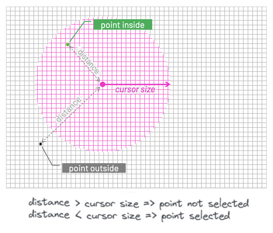
We could square root the squared distance and then compare cursorToPosDist to cursorSize. But multiplying two numbers is a less performance-demanding operation than calling the expensive sqrt function, so we saved ourselves a few CPU cycles here. That is good, especially since the Update function is called every frame. Such code is sometimes called a "hot" code because it's executed many times. The opposite would be cold code, which is for example our Setup function, which is executed only once, at the beginning.

Vec2 cursorToPosDir = pos - mouse->GetPosition();
float cursorToPosDist = cursorToPosDir.x * cursorToPosDir.x + cursorToPosDir.y * cursorToPosDir.y;
float cursorSize = mouse->GetCursorSize();
isSelected = cursorToPosDist < cursorSize * cursorSize;

We set the isSelected flag also in the stick. This would be one or two sticks, depending on how many are associated with a particular point. That's why we keep pointers to them in the array sticks[2].

for (Stick* stick : sticks) {
  if (stick != nullptr) {
    stick->SetIsSelected(isSelected);
  }
}

Next, we check if the left mouse button is pressed and the point is selected. If so, we get the difference between the current mouse cursor position and the position the cursor had in the previous frame, and we set the previous position of the point to the difference between the current position and the difference between cursor positions we've just calculated.

When it comes to Verlet integration at the bottom of this function, the difference added to the previous position of the point acts as if we added a force to the point in the direction we move the cursor.

The faster we move the cursor, the bigger the difference and the force will be. Unless it's outside the bounds of this elasticity value; if so, we simply cap the difference to elasticity or minus elasticity, according to the direction.

if (mouse->GetLeftButtonDown() && isSelected) {
  Vec2 difference = mouse->GetPosition() - mouse->GetPreviousPosition();
  if (difference.x > elasticity) difference.x = elasticity;
  if (difference.y > elasticity) difference.y = elasticity;
  if (difference.x < -elasticity) difference.x = -elasticity;
  if (difference.y < -elasticity) difference.y = -elasticity;
  prevPos = pos - difference;
}

When the user presses the right button, and similar condition is met, we simply break the constraints associated to the selected point, leaving a tear in our cloth.

if (mouse->GetRightMouseButton() && isSelected) {
  for (Stick* stick : sticks) {
    if (stick != nullptr) {
      stick->Break();
    }
  }
}

The last piece of the puzzle is the Stick class. The good news is that this one is actually much more simple than the Point class. We can see in the Stick.h header file that we keep references to a pair of points to which a stick is connected, as well as the length that should be maintained by the constraint.

We also have flags for isActive and isSelected. We set sticks to inactive in the Break function, and we just saw how we set the selection of sticks via the SetIsSelected function when we update the points.

Finally, sticks are the things we want to see rendered on the screen. Therefore, we pass a pointer to SDL renderer to our Draw function, and we also store the stick colors here. One regular color and another color for when the sticks are selected (inside the cursor circle). Both colors are stored as a hexadecimal number of Uint32 type in ARGB color format.

#include "Renderer.h"

class Point;

class Stick {
  private:
    Point& p0;
    Point& p1;
    float length;

    bool isActive = true;
    bool isSelected = false;

    Uint32 color = 0xFF000000;
    Uint32 colorWhenSelected = 0xFFCC0000;

  public:
    Stick(Point& p0, Point& p1, float lenght);
    ~Stick() = default;
    void SetIsSelected(bool value);
    void Update();
    void Draw(const Renderer* renderer) const;
    void Break();
};

In the Update function of Stick.cpp we can see how we maintain the distance between active points. This is not new for us, we've already seen that in the p5.js example. The logic is pretty much the same.

void Stick::Update() {
  if (!isActive)
    return;
  
  Vec2 p0Pos = p0.GetPosition();
  Vec2 p1Pos = p1.GetPosition();

  Vec2 diff = p0Pos - p1Pos;
  float dist = sqrtf(diff.x * diff.x + diff.y * diff.y);
  float diffFactor = (length - dist) / dist;
  Vec2 offset = diff * diffFactor * 0.5f;

  p0.SetPosition(p0Pos.x + offset.x, p0Pos.y + offset.y);
  p1.SetPosition(p1Pos.x - offset.x, p1Pos.y - offset.y);
}

In the Draw function, we render the stick using our wrapper around the SDL window and renderer. This is simply done by drawing a line from one point to another. Normal color when the point is not selected, and red when it is.

void Stick::Draw(const Renderer* renderer) const {
  if (!isActive)
    return;

  Vec2 p0Pos = p0.GetPosition();
  Vec2 p1Pos = p1.GetPosition();

  renderer->DrawLine(p0Pos.x, p0Pos.y, p1Pos.x, p1Pos.y, isSelected ? colorWhenSelected : color);
}

And that's it! We have our 2D cloth simulation working.

Final Considerations

This concludes our implementation. There's a lot packed in this article; if you got to the end of it and managed to get your version of the cloth simulation working, kudos to you! This is no small achievement.

As always, more than just seeing something moving on the screen, I hope you enjoyed diving into the theory and especially the math topics that we discussed. We touched a little bit of differentiation, integration, different numerical methods, JavaScript, C++, SDL, and so much more.

If you want a small challenge at the end, download this GitHub repository and try to implement "tearing by distance". In other words, the constraint between the points will break if the distance between those points extends a certain value.

If you have any suggestions for this article, you can always contact me and also follow me on Twitter. It will be great to see you there.

---